Example of an algorithm development process

Consider the task of measuring of the grain size for the image of the ferrite grains

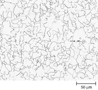
The image "FerriteGrainBoundaries.tif" is a courtesy of PELM centre, Central Queensland University, Gladstone, QLD, Australia.

Open empty Pictorial Image Processor project and perform spatial calibration

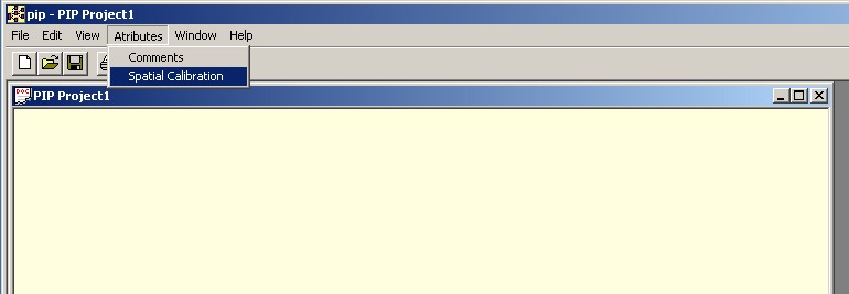
In the Spatial Calibration Dialog

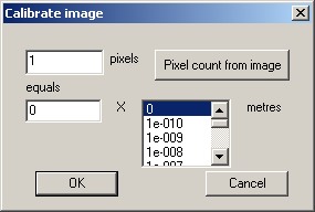
press "Pixel count from image" button. In the appearing File Open dialog select the calibration image, in this case "FerriteGrainBoundaries.tif", the source image. Obtain the pixel count line from the image following the ruler present in the image,

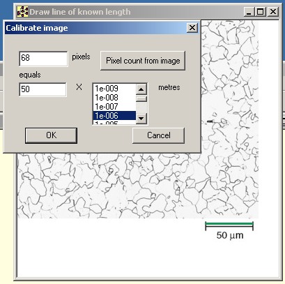
enter the corresponding world coordinates and multiplier to obtain the calibration in meters. Press OK. Background of the project window changes indicating that the project is now calibrated.

Open the source image "FerriteGrainBoundaries.tif" in the project window. We recommend avoiding jpeg images in algorithm development because interpolations introduced by the lossy compression will add another source of confusion, image decoded by the Pictorial Image Processor jpeg library can be different from the image decoded by other library and may in detail look different if open say in Photoshop. Quick look at the image shows that simple thresholding operation will not delineate the grains correctly because some of the grain boundaries are stronger than others and simple thresholding will not be able to preserve connectivity. To check that use for example SIS automated thresholding technique.

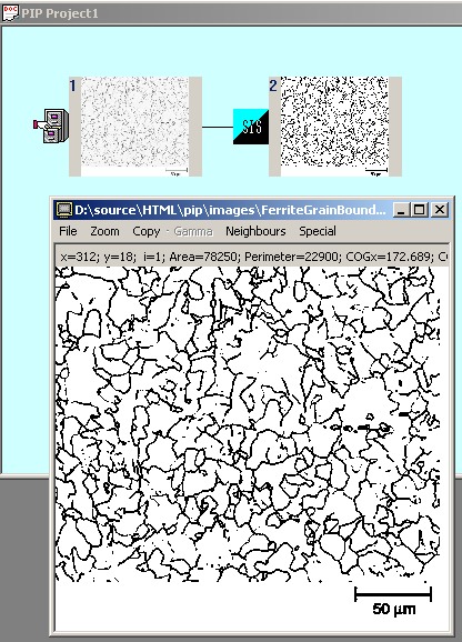
In this image some grains have fused because the intensity of grain boundaries in the original image were not constant. For the same reason after thresholding the boundaries have varying thickness. Attempt to count the number of grains using labeling operation will lead to incorrectly small number.

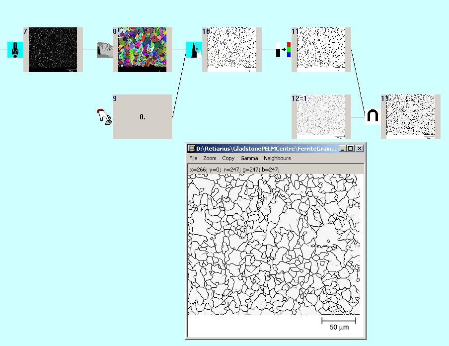
It is known in the image analysis that a more robust method for blob separation is so called watershed procedure. It is also known that the watershed can suffer from over-segmentation if the image has intensity variations cased by the noise in the image capture equipment. Random fluctuation of the intensity can cause the method to build the "dam" on the noise speck as well as on the image feature. The sketch of the algorithm below with the resulting image displayed in Full Size View illustrates the over-segmentation.

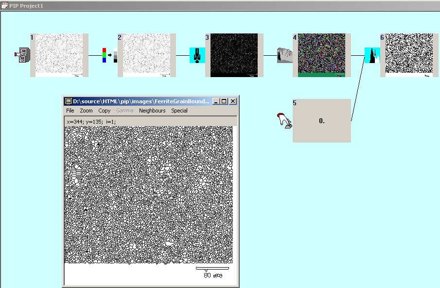
The sequence of the operations in the algorithm above is as follows: at first source image is converted to a grey scale image from the original RGB(operand 2), then inverted (3) since watershed will "flood" the dark,grain areas building the "dams" along the bright, edge areas, then watershed is applied (4), then image is thresholded above 0 to obtain the boundaries as the background and grains as the foreground intensity. In Pictorial Image Processor watershed operation marks connected "flooded" areas with non-zero intensities presented as different colours while the "dam" lines are marked with the intensity 0, black. Last operation (6) groups all non-zero intensities into a single foreground intensity 1.

The example above indicates prior to application of the watershed method the image has to be preprocessed in order to suppress the noise while preserving the features. For our source image which is essentially black and white with the key features on the opposite sides of the intensity range the best noise suppression technique could be median filter.

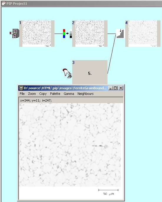
By itself median filtering is not providing good grain delineation because it suppresses the grain boundaries. In order to recover them we apply morphological reconstruction operation to the grey scale image (2) using filtered image (4) as the marker. Median filtering will smooth out small peaks in both intensity up and intensity down directions. Subsequent reconstruction will recover the intensity down peaks but intensity up peaks and their surroundings will be capped by the median filtered image.

The resulting algorithm can be presented in next 2 pictures, second picture continuing the first and operand 7 present on both pictures to show the link point. Operand 6 is the result of the reconstruction. Operand 11, conversion to RGB image is facilitating overlay of the results over the original.

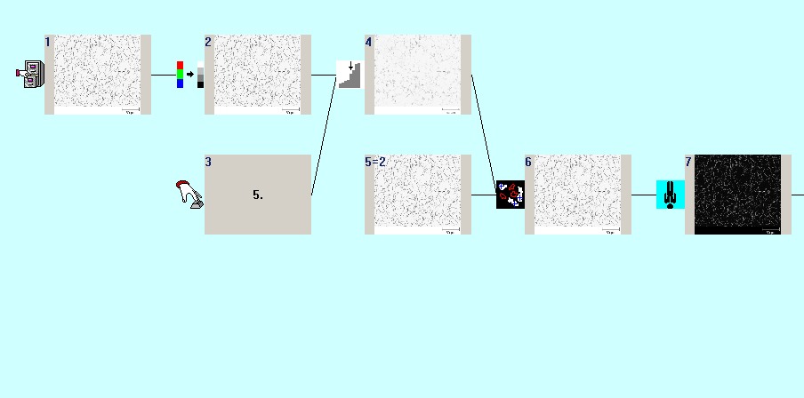
On the second picture apart from the algorithm operands we presented the full size view of the operand where the original image is overlaid with the black lines of the grain network found.